All the material presented in these methodological articles, but with more details, can be found in the book Option Fair Value: Finding a Statistical Edge in Options Trading. A free copy is available for registered users.
Fair Value implies the historical fairness of an option price. The key here — historical. Actually, we calculate an option price at which both buyer and seller have had zero profit on average for some period in the past. Then, we treat this price as a Fair Value that is expected to realize after some number of trades in the future.
The question is whether or not we can trust this number and rely on such an extrapolation. Yes, of course, but not blindly. Like any statistics calculated based on observed outcomes, Fair Value is not an exact predictor with 100% guarantee. However, we have no other data other than that observed in the past, and we can operate with it, anyway.
At first, we have to estimate the prediction power of this value (one method is to calculate confidence intervals for it). Then, we can try to reduce the variance of future results by the filtering technique presented below.
So, the Fair Value of a derivative is based on the underlying security behavior in the past. The reasonable question is whether we can rely on this past to base our expectations for the future? The answer is yes if we
extrapolate to the future only the past that resembles the present
In other words, we should select from the past only those days in which the market was in the condition similar to the current state. That is a filtering idea, in brief.
As opposed to the classic hypothesis of the market prices Random Walk (that has been disproved by various research works and the science of behavioral finance), the OptionSmile methodology is based on the assumption that
markets live within distinct regimes
The main idea is to get some numerical indicator of a current regime and select from the past only those dates when such an indicator had similar value; then, calculate the Fair Value based on the market behavior only in those dates.
There are many types regimes to identify. In this article, three of them are discussed below:
It is well-known that market volatility is not randomly distributed, but “clustered” by the distinct volatility regimes. Obviously, rather prolonged periods of either low or high volatility occur, and it is not wise to derive the options Fair Va`lues from both of these periods as from one distinct dataset. We would get a “mixed bag” of regimes.
Volatility levels can be spotted by two types of indicators:
The historical, or realized, volatility is lagging in nature and grasps the state that has already passed, while the volatility implied by options prices is forward-looking and is preferable for our filtering purpose.
Because we have values of the volatility indicator (e.g., VIX) for each day in the past, we could group all those days to some “bins” with some VIX range; for instance, 0-14, 14-18, 18-25, etc. These bins would represent subsets of days with different volatility regimes: low, medium, high, etc. Each of these subsets must be analyzed independently, and options Fair Values should be calculated based on each dataset separately.
Here is an example of the market historical mispricing for the 2-week put options on SPY, for two volatility regimes: low volatility (VIX < 14) and high volatility (VIX > 18). The data range has been taken from October 2009 to October 2017, i.e., 8 years of the secular bull market; both segments (we call them Filter Bins) comprise 653 and 695 days respectively.
The blue lines show the Fair Values, and the red lines demonstrate the average historical market prices estimated according to our methodology.
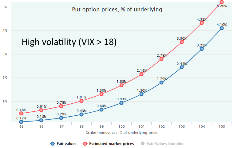
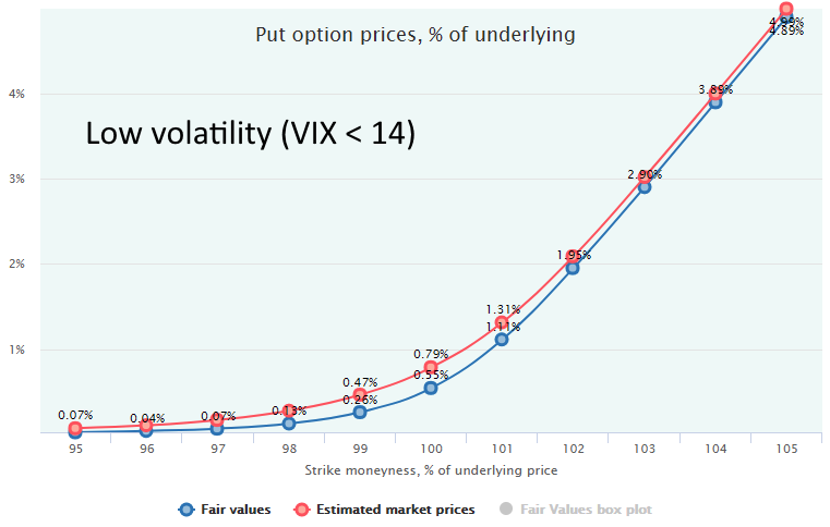
Obviously, the discrepancy between Fair Values and Market Prices is much bigger in high volatility periods. It confirms the fact that the market in “panic mode” tends to overestimate future volatility by far. Even though realized volatility (standard deviation of returns) for such periods has been also higher (annualized 16.8% when VIX > 18 vs 8.3% when VIX < 14), the market participants tend to overreact to it and push the prices of put options even higher than it is justified by the market behavior that follows. Here the sellers of put options have an edge and a rather high expected profit.
In the low volatility regimes, the market has been valuing the put options rather fairly. The difference between Fair Value and Estimated Market Prices is not significant.
For more about the filtering by volatility, see our research: Options Mispricing in Different Volatility Regimes. Another research is devoted to the systematical puts overpricing, see Are puts really overpriced?
This idea based on the assumption that security prices behave differently in different so-called “secular markets” (bull, bear, or rangebound) that last for some prolonged time, usually years, or even decades. In all such cycles, markets have different price patterns. For example, in the bull markets, almost all downward corrections are finally bailed-out, and prices continue their way up. The bear markets exhibit the opposite behavior: on the way down, there are some upward corrections (“dead cat bounces”) that are finally interrupted by the continuation of the downward move.
For the options pricing, all that leads to the very different probabilities of expiration in-the-money that constitutes their Fair Value. Remember, it is a mathematically expected payoff at expiration calculated as a probability-weighted payoff function. For instance, if a market trends downward, the probability of a put option to expire ITM is much higher than in an uptrending market. The opposite is true for calls.
There are many ways to spot the long-term direction of the market. Here are just some of them:
Here is the chart of the S&P 500 Index for 20 years. It is easy to manually spot the distinct periods when the market was trending up (5 periods), down (2 periods), of fluctuating within some range (5 periods).
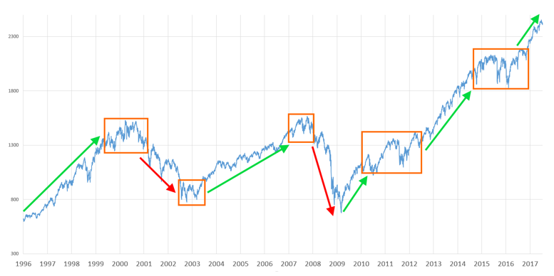
We can group all the periods by their type and calculate the Fair Values, Market Prices, and market mispricing for each group separately. To find a current mispricing, we will compare the real-time market prices strictly with the Fair Values for the regime similar to the current: bull, bear or rangebound.
There are many drawbacks of such an approach, of course. First, different analysts will come up with the different breakdowns by the regimes looking at the same chart; it is more an art than a science. Second, all the regimes inevitably overlap each other. For example, the start of a new prolonged move, either up or down, occurs within some rangebound market. In such cases, it is safe to adhere to the conservative positions and “mix” two periods into one Filter Bin.
Besides this manual approach, it is possible to employ more algorithmic methods with various technical indicators supposed to signal the trend inception, such as Price Channel, Moving averages, etc.
Perhaps, the most popular way to spot a directional market regime is to use moving average (MA) indicators. There are innumerable methods of trends identification with them and one of the most popular is a Long/Short MA crossover. It involves the calculation of two moving averages: long-term (say, 200 days) and short-term (say, 50 days). Technical analysis asserts that if the Short MA crosses up the Long MA from below, it means that a new uptrend begins and a buy signal is generated. If this crossing happens downward (so-called “death cross”), a new bear market starts, and a sell signal takes place. Respectively, if Short MA is above Long MA, we are in the uptrending regime. The opposite position of moving averages implies that the market is downtrending.
Here is the same chart of the S&P 500 index with two simple moving averages (SMA) overlays: Long SMA for 200 days and Short SMA for 50 days.
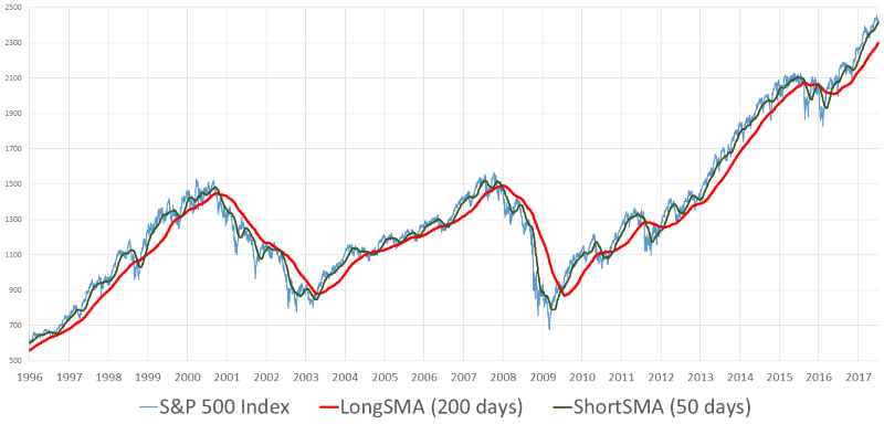
It is easy to spot the major bull and bear markets similar to the ones identified manually, but periods of rangebound markets are not easy to highlight on this chart. The obvious advantage of using technical indicators for filtering is that they point to the market state rather clear and without ambiguity, i.e., they explicitly state what exact trend we have right now.
In the long run, the prices in financial markets follow the underlying fundamentals that a security represents. For stock markets, it is a phase of the economic cycle. In particular, bear markets are always the consequence of economic downturns, namely, recessions that can be identified and filtered out by the various macroeconomic indicators.
There are numerous indicators aimed at the recession prediction that can be exploited to filter out these periods from historical data. The most valuable are so-called leading economic indicators that are good at grasping the current economic conditions before the release of the official GDP data that is deemed as a lagging indicator. Some examples are as follows: Purchasing Managers Index (PMI), ISM Manufacturing Index, credit conditions, various labor market indicators, credit spreads, and others.
All these indices capture some aspects of the economy, and being combined into the one composite index of leading indicators can predict the future economic conditions with quite an appropriate degree of certainty.
For example, one of the most popular composite indicators is the Leading Economic Index® (LEI) calculated and published monthly by The Conference Board. It incorporates 10 different gauges of the US economy reflecting labor market conditions, new orders, real estate market indicators, stock market, credit conditions, interest rate spreads, and consumer expectations.
This indicator is quite good at the downturns prediction, as it usually starts to decline around 3-6 months before the actual recession and, hence, predicts the bear market.
Here is the overlay of LEI over the S&P 500 index and the actual recessions (shaded areas):
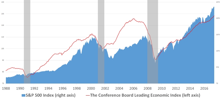
It can be observed how good this index was at predicting the economic downturns and the respective bear markets. It was beginning to decline in several months or quarters before the stock market started to price-in the approaching recession.
For our purpose of filtering out the bear markets from historical data, we can calculate the Rate-of-Change (ROC) indicator that simply shows the rate of increase or decrease of this index for some period, say 3 or 6 months. Should this indicator fall below some threshold value, i.e., 2%, that would indicate the bear market conditions. Returning to the area above this level would mean the end of the recession and the bear market.
Here are the highlighted periods when 6-month ROC was below 2%.

The following chart reveals the huge discrepancy between the Fair Values of 4-week put options on SPY for the downturn periods, when the 6-month ROC was below 2%, and other times when this indicator was above this threshold.
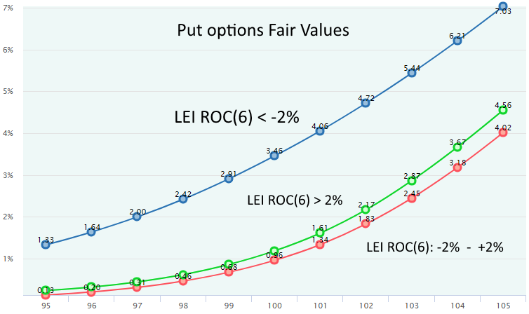
Interestingly, this indicator is not good at distinguishing between bull and rangebound markets. Nevertheless, it is useful to filter out the recessions and vivid bear markets from the historical data set. It is necessary to do because its inclusion brings a significant distortion into the Fair Value calculation. For example, the probability of ITM expiration of a 4-week put with 96 moneyness is 34% in the bear markets and 9.4% in other periods. So, the Fair Value of this particular contract is 1.64% and 0.26% respectively, the six-fold difference.
Here is how the options market have valued these put options (we take only OTM side with moneyness < 100).
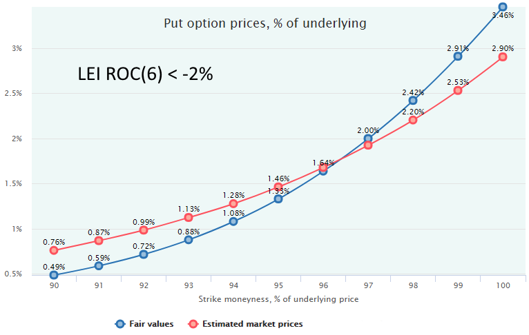
Here we see that in the recessionary environment, put options are rather close to their Fair Values: slightly undervalued near-the-money and overvalued farther OTM, perhaps, due to the huge demand for insurance on the negative tail.
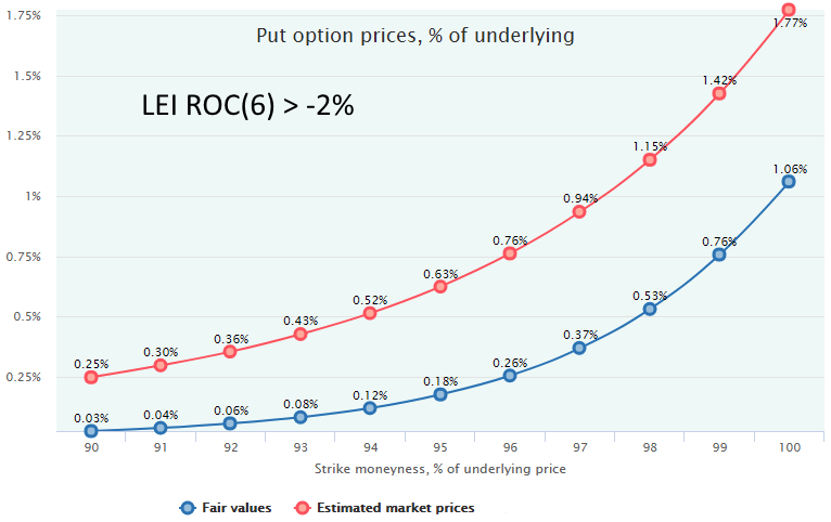
In all other periods (see below), the options market tends to hugely overestimate put options. So, in times when there are no signs of an economic recession approaching, the sellers of put options have a significant edge and a rather big expected profit. In contrast, the put buyers have a large expected loss, and buying puts as an insurance for a long portfolio impose a substantial drag to the overall performance.
For more about the put options overpricing, see our research: Are puts really overpriced?
Every “market” — either bull, bear, or rangebound — can be further sliced into the short-term segments when the market also demonstrates some repetitive patterns lasting in the timeframe from one week to several months.
Even though such fluctuations are much more random than the long-term trends caused by economic fundamentals, it is possible to find some distinct patterns, calculate the options Fair Values, and analyze market mispricing.
There are many so-called “swing trading” methods, techniques, and indicators invented in attempts to utilize such types of non-randomness of the market. Technical indicators are, perhaps, the most suitable for the purpose of the historical data filtering. Some examples are:
Those who believe in the prediction power of these indicators (technical analysts) have developed numerous rules, according to which signals to buy or sell a security are generated. There is no lack of books, web resources, software on this topic.
In the OptionSmile methodology, those indicators are helpful not as a signal generating tools but as a mean of the historical data filtering. Namely, we can take a “snapshot” of the current market condition with some indicator and select from the past only those days when
this particular indicator was in some range around that current value
Then, the Fair Value of options and the market prices are calculated only on the basis of this data subset. Pretty much the same as the filtering by the Volatility Index or Macroeconomic Indicators.
Below is an example with the Relative Strength Indicator (RSI) capturing the position of the current price of a security relative to the prices in some period in the past. It is often used as a mean-reversion tool capable to identify how far the market has gone from some average levels. It is assumed that a relatively low level of RSI signals that the market is “oversold” and is ready to bounce up, and a high RSI says the market has gone up too far (“overbought”) and a correction downward is approaching.
In this example, we have used 2-week options on SPY and have taken the 20-year period from October 1997 to October 2017. Without volatility filtering, but with exclusion of the recessions and bear markets with the Leading Economic Indicators 6-month Rate-of-Change (filtering out all the days with LEI ROC < -2%):
We take the RSI for 14 days as the most popular interval and split all data into 3 Filter Bins:
Usually, the upper and the lower thresholds are taken as 30 and 70, respectively. But such levels would leave us with too small number of days.
Here are the statistics of the 2-week underlying returns (SPY) for these bins. Bin 0 is without RSI filtering.

There is an obvious striking difference between average return in periods with RSI<40 and all other periods, including the whole dataset (bin 0). Mean return is 1.57% (39.7% annualized) while unfiltered mean return is 0.51% (12.8% annualized). Obviously, the mean-reversion force is rather strong in such an “oversold” regime. That conclusion supports the fact that the buying of oversold markets (“buying the dips”) has been a very profitable strategy during the secular bull markets.
On the opposite side, in the “overbought” regime (Bin 3, RSI > 60), the mean-reversion force does not reveal itself. Even though the market has been already going up for some time, it does not exhibit a sharp downward correction right after that, on average.
That was a brief overview of the SPY behavior. Now let’s look at the options markets.
Here is the options mispricing in the Bin 1:
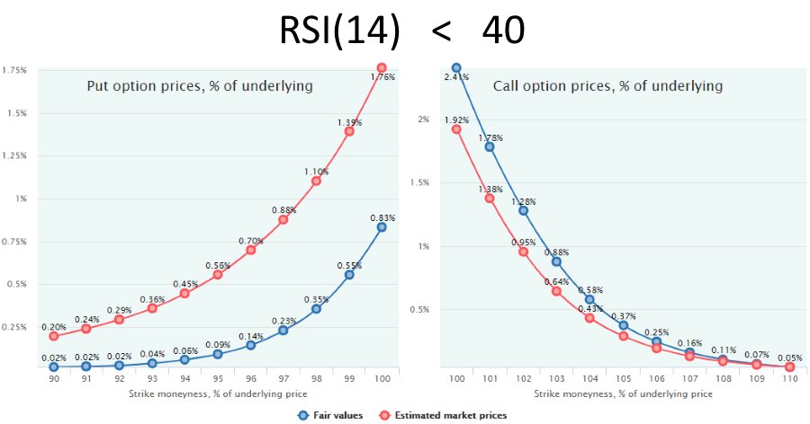
Obviously, the put options are hugely overpriced in this regime, and there are two sources of it:
These two factors combined produce such a substantial put options overpricing.
The optimal strategy for such a market regime (besides outright buying of SPY) would be the Bullish Risk Reversal: selling puts, buying calls. That strategy would have a rather high expected profit: for example, selling the 99 put (for 1.39%) and buying the 101 call (for 1.38%) would give an expected profit of 1.24% (more about the metrics of the options combinations, see Fair Value of Options Strategies).
Of course, such a strategy of “catching the falling knife” is also quite risky and is not for everyone. The profit volatility is also rather high, and strong trading discipline with the good money management technique is necessary to observe the future realization of such a high expected profit.
Bin 2 comprises the days in history when the market had not gone far from the prices levels of the recent weeks.
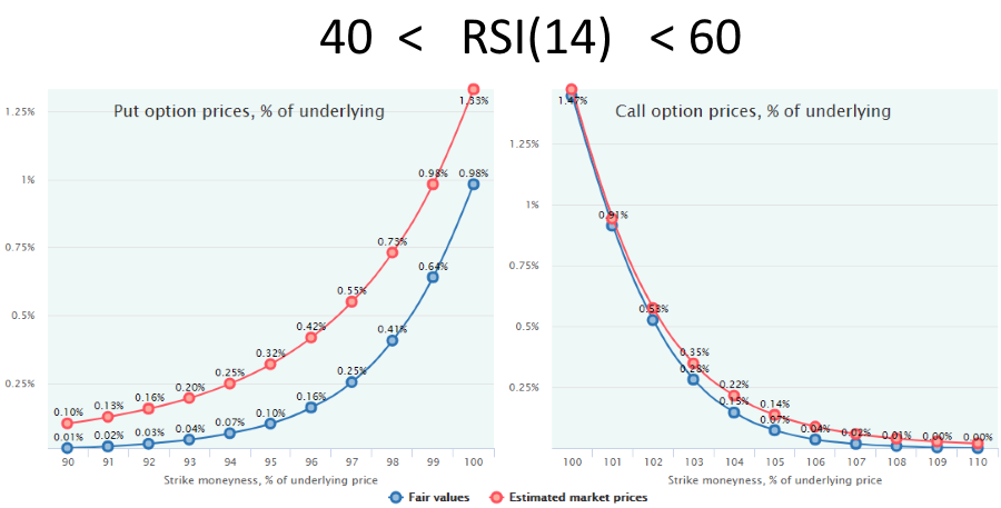
Here, the put options are still overpriced although not as much as in Bin 1. More interesting is the call side where the options are valued rather fair, especially near-the-money. That means neither buyer nor seller have any substantial edge over each other. Their expected profit does do not differ significantly from zero.
The best strategy here would be to stay away from the calls and sell puts or put spreads.
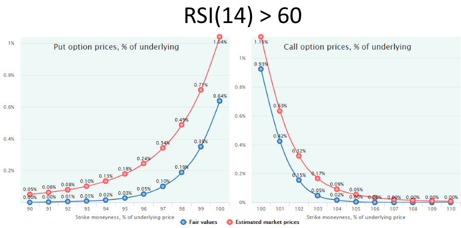
The put options are, again, overvalued (they are systematically overpriced for stock indices, see our research Are puts really overpriced?).
However, on the call side, the results are rather confusing at first glance. On the one hand, the market shows a positive average return on these periods (0.29% for 2 weeks), which should lead to the profitability of buying of the call options instead of selling them. On the other hand, this chart shows that this is a losing strategy because the Fair Value of call options is less than the average market price. On the contrary, selling calls should be profitable.
That rather strange outcome could be explained by the specific pattern the market demonstrates in the secular bull markets. After some time of trending up, the market becomes exhausted, but it is not followed by a massive, prolonged correction that would lift puts Fair Values. At the same time, the market does not have enough steam to go further upward and to increase calls Fair Values. Instead of that, it fluctuates for some time on the level achieved. Hence, the most profitable strategy in such a market would be selling both puts and calls (short straddle, strangle, iron condor, etc.).
Another important implication of this example relates to such popular strategy as Covered Call: selling calls against the long underlying. Our research shows that for the stock indices the call options are priced rather fairly by the market (excluding recessions and bear markets), in contrast to the overvalued puts.
That makes the Covered Call strategy almost worthless if done mechanically: all the premium collected by call selling will eventually be lost in the form of not participating in the growth of the underlying security being called-out. So, the call’s premium collected can be considered just as a form of cash dividends but not as an extra income. In addition, a covered call has less volatility than an outright buying of the underlying security.
However, we could act tactically and filter out the market regimes when the call options are underpriced and selling them would have an expected loss (see Filter Bin 1, oversold market). In this case, these short calls would not pose a drag to our portfolio.
Here, we have seen that different short-term regimes make one strategy profitable and another losing — in terms of their mathematically expected result that is not guaranteed in each particular trade, but it can be treated as an average profit/loss to which the final result is supposed to converge after some number of trades.
By calculating the Fair Value, we are trying to calculate an options price that will realize in future as an “equilibrium” price providing zero average profit for a buyer and a seller. Filtering of the market regimes is a technique that makes such a prediction more reliable with less variance of results.
Such a technique can be compared with the weather prediction for some geographical location (underlying security, in our case). If we know just the name of a city and its location, we can somehow predict the air temperature for some moment for tomorrow, but with a huge margin of error.
However, having more information about the current season and the average historical temperature in this particular month for this area, we can make our prediction more reliable. By adding to this some historical data of the average temperature at the time of the day for our future point (day, morning, evening, night), as well as our knowledge of the current weather conditions (rainy, cloudy, sunny, storm, etc.) we can make our forecast even more solid.
In our case, the season is the analogy of the long-term cycle (bear, bull, rangebound), the time of the day is similar to the short-term market regime, and the current weather conditions are like the market volatility. We extrapolate to the future only those dates in the past that were similar to the current market condition.
Read next: Fair Value Confidence Intervals