The Fair Value of an option is actually the current value of expected payoff of a contract at its expiration. Mathematically speaking, an expected value is always calculated by weighting of all possible outcomes by their probabilities.
The key property of such a formula, using the arithmetic average, is that it does not take into account the compounding effect of the previous returns. In other words, the Fair Value of options assumes that the profit/losses of all the hypothetical “trades” are not capitalized, and one particular outcome does not influence the “magnitude” on the next trade. The basis of each trade is the initial portfolio value and does not change during the whole experiment.
That is not exactly what happens in real trading, of course. Usually, the result of a trade is accrued on the portfolio and the size of the next trade is calculated on the new basis – including the previous results. That requires a new dimension of the strategy development, which is usually called Money management or Position sizing.
In this post, we discuss the influence of the returns compounding on the final results and observe all the instruments provided by the OptionSmile platform to deal with the volatility impact.
It is well known that, in case of returns compounding, the volatility of a strategy can harm the final total result. Having positive mathematical expectation (arithmetical average) but unstable returns, it is possible to ruin the whole portfolio. For instance, having lost 50%, it is necessary to gain 100% to break even.
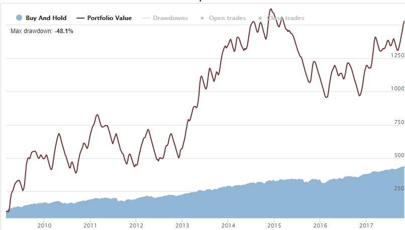
See the example of XIV ETF, which had lost about 23.5% of its value in 2014-2015 while having a positive daily average return of 0.03% (+7.2% annualized):
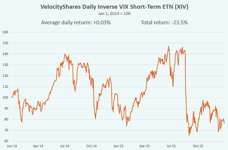
That mathematical phenomenon is often called the “volatility drag” that makes the geometric average returns always less than the arithmetic average if the variance of returns is greater than zero. If all returns are compounded, the geometrical mean is actually what builds the final portfolio value at the end.
Many inverse and leveraged ETFs also suffer from the volatility due to the daily rebalancing and compounding – to maintain their leverage ratios constant. Having huge volatility, especially in leveraged ETFs, those products can be the great value destroyers despite the positive mathematical expectations.
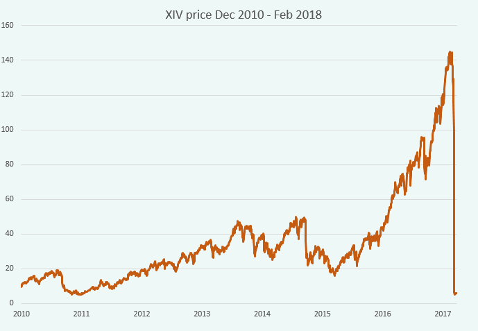
Update as of Feb 2018:
XIV fund collapsed on February 5, 2018, after the huge VIX spike (up to the 50th levels). The value of the fund had dropped from 140 levels to 6 in just a couple of days. The reason for this is the requirement for the daily rebalancing of their holding of short VIX futures. They simply were forced to liquidate this massive of short futures and accrue the loss on the portfolio (-75% on Feb 5), which is non-recoverable in future. This is the same phenomenon that we discuss in this article:
The OptionSmile platform has all necessary tools and indicators to identify and quantify that volatility drag and find the right instruments to fight it.
Finding the mathematical expectation of an option payoff – its Fair Value – and comparing it with the Market Price is just the starting point of a strategy development. Having positive expected returns is the minimum requirement for the profitable result. In fact, with the expected loss, it is impossible to reach a positive total portfolio gain with any volatility level, even zero.
Having the Fair Value exceeding the Market Price or vice versa for short positions, we get a positive Expected Profit/Loss and, hence, the positive Return on Margin (for margin positions) or Return on Market Value (for non-marginal positions) – see the performance metrics workflow in the Tutorial.
The next step is to make a decision about the portfolio share we are going to put on risk. In other words, we should set the Position Size parameter (two indicators – Kelly criterion and Optimal Position Size to assist in this choice), and get the Return on Portfolio metric, which is still calculated as an arithmetic average.
Finally, to get an indication of the total return with compounding, the Geometric Average Return on Portfolio is calculated. The difference between these two Returns on Portfolio (arithmetic and Geometric) can be considered as an indication of the abovementioned volatility drag. Its size is the direct outcome of the Position Size parameter: the greater the portfolio share we put on risk, the bigger is the discrepancy between the arithmetic and geometric returns.
Here is an example of the simple Long Call strategy with 20-day at-the-money options on SPY in the Bull Market of March 2009 – November 2017. The key performance metrics – before the Return on Portfolio – are the following:
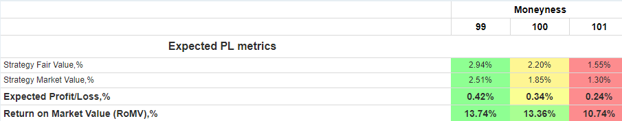
As we see, the strategy of calls buying has been profitable on average on that Bull Market.
However, if we bought these options on the whole portfolio, we would have lost all out money quickly (in case of compounding). For example, here are the average Returns on Portfolio – arithmetic and geometric – with 100% Position Size:
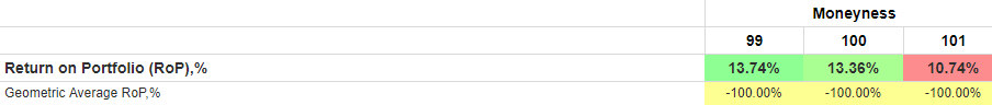
Geometrical Average RoM indicates that we have lost all the money while having the positive expected (arithmetic) Return on Portfolio. The strategy dashboard for 100 moneyness Long Call indicated we had done in very quickly – in June 2010 we ended up with zero portfolio value:
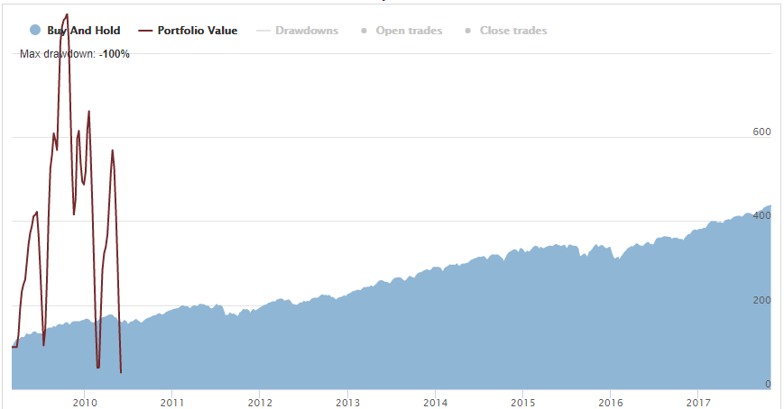
It is obviously the result of the “overbetting” (setting too big position size) and the volatility drag which has ruined the whole portfolio.
The detrimental volatility effect still persists in 50% Position Size:
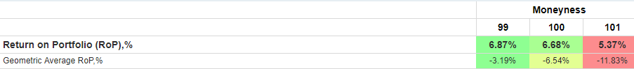
With this position sizing, our portfolio had approached zero in late 2015:
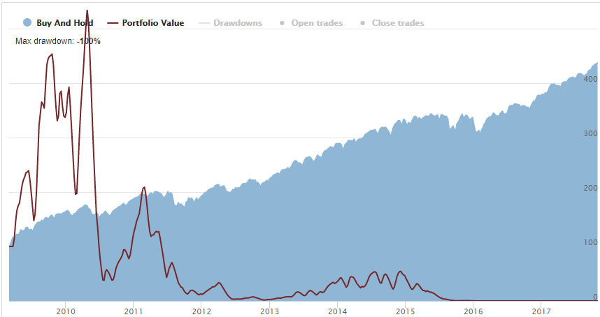
It is still overbetting, obviously.
What is the optimal position size then? Not too low to provide enough return and not too big to destroy the portfolio by overbetting.
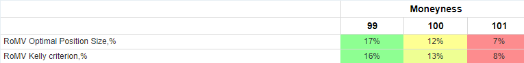
The OptioSmile strategy performance metrics has two indicators to assist in this task: Kelly criterion and Optimal Position Size. Both of them do the same job: they calculate a position size that maximizes the total return. The second one is more suitable for our purpose since it directly maximizes the Gometrical return. For details, see here.
For our Long Call strategy, the following optimal values are calculated:
For the startegy with 100 moneyness here is how Geometric Average return (vertical axis) looks like depending on position size (horisontal axis):
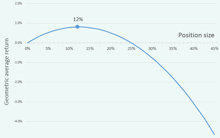
So, the best sizing parameters for 100 Long Call is 12% – that value provide maximum Geometric average return (notice how it turns negative after 25% position size). And with Portfolio Size of 12% we get the following results:
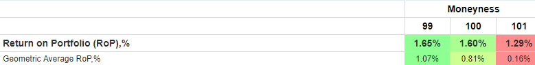
The Geometric return has finally become positive and our portfolio has not lost money. Here is the equity line for 100 moneyness:
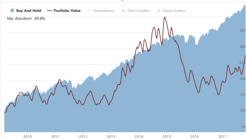
Not a quite impressive performance but at least not losing money.
Note that Buy&Hold strategy has had higher terminal portfolio value at the end than our Long Call strategy even with the “best” portfolio sizing.
It turns out that for this period (2009-2017), no position sizing parameter exists that would allow an ATM LongCall strategy (with compounding) earn more than a simple Byu&Hold strategy. Even though it has higher mathematically expected return (with 100% position sizing – much higher) than the Byu&Hold has.
However, there is always a possibility to refrain from the compounding of returns and stay in the arithmetic average paradigm. In this case, we set the initial total portfolio value, the position size parameter, and (by multiplying these two) the sum of money we are going to put on risk. That amount should be kept constant disregarding the previous returns and the resulting portfolio value.
Here is the same 100 Long Call strategy equity curve with 100% position sizing but without compounding:
This has changed the whole picture. The equity line is still not so pretty and has vivid plateaus and big drawdowns, but it completely differs from the variant with compounding.
It is necessary to note that in this approach, the share of portfolio at risk – in percentage term – will be floating depending on the previous results. In case of profit accumulation that ratio will decrease, and, if we get losses, it will increase. For example, in some extreme situation, having position size of 50% and suffering a loss of 50% of the portfolio, we have to put at risk the whole remaining half (100% Position size) to keep the absolute amount of money at risk constant.
Nevertheless, in some strategies, such as discussed above, the profit/loss accumulation without compounding can produce superior results relative to a strategy that capitalizes all the returns.
In any case, the OptionSmile platform has the whole arsenal of various tools to identify the proper parameters for an options trading or hedging strategy.